Plate Heat Exchanger Model
The advanced ice storage model implemented in the CTI project “Modul-Ice” extends the capabilities of Polysun to represent different kinds of ice storages. While the existing model relies on an empirical fitting function fixed to the specific kind of coil heat exchanger geometry used in Viessmann-Isocal ice storages, the new model was designed to simulate any ice storage with plate heat exchangers. The heat exchanger material and geometry as well as the distance between heat exchangers in the ice storage can be parametrized.
Symbols and Nomenclature
| \(UA_{tot,i}\) | overall heat transfer coefficient times surface area product of one heat exchanger temperature node, W/K |
| \(UA_{in,i}\) | internal heat transfer coefficient times surface area product of one heat exchanger temperature node, W/K |
| \(UA_{wall,i}\) | wall heat transfer coefficient times surface area product of one heat exchanger temperature node, W/K3 |
| \(UA_{ice,i}\) | ice heat transfer coefficient times surface area product of one heat exchanger temperature node, W/K |
| \(UA_{out,i}\) | external heat transfer coefficient times surface area product of one heat exchanger temperature node, W/K |
| \(Nu\) | Nusselt number [-] |
| \(Re\) | Reynolds number [-] |
| \(\Pr\) | Prandtl number [-] |
| \(d_{h}\) | hydraulic diameter [m] |
| \(b\) | width flow cross section [m] |
| \(A\) | area of one control volume [m2] |
| \(\lambda_{fluid}\) | heat conductivity fluid [W/(K m)] |
| \(x_{wall}\) | wall thickness [m] |
| \(\beta\) | coefficient of thermal expansion [m/K] |
| \(\rho\) | density [kg/m3] |
| \(l_{c}\) | characteristic length [m] |
| \(c_{p}\) | specific heat capacity [J/(kg K] |
| \(\mu\) | dynamic viscosity [kg/(m s)] |
| \(Ra\) | rayleigh number [-] |
| \(x_{ice}\) | ice thickness [m] |
| \(Q_{hx}\) | heat exchanged between heat exchanger and storage [J] |
| \(\Delta H\) | enthalpy of fusion [J/kg] |
Model design
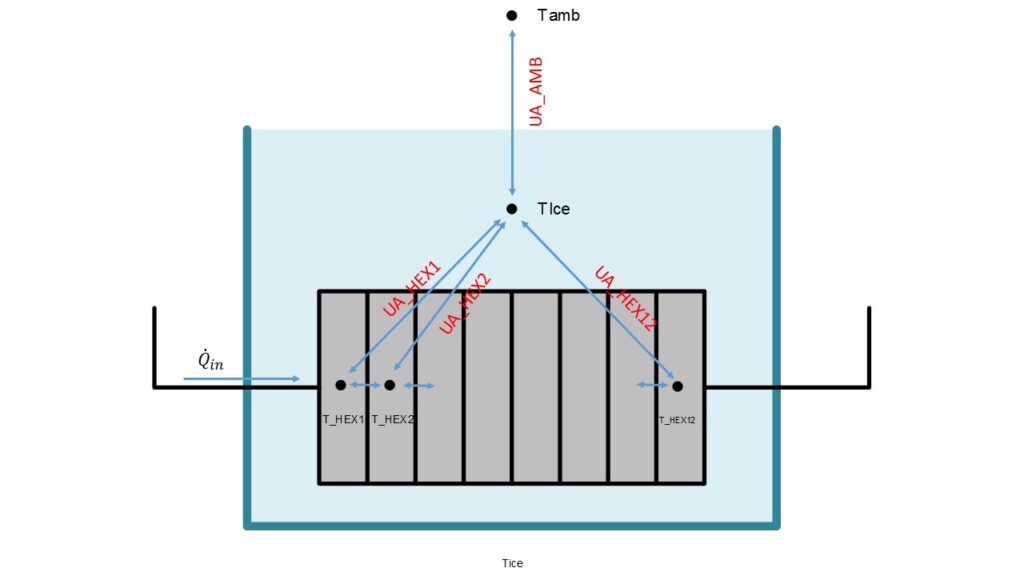
The Model is based on discrete control volumes with the corresponding heat transfer equations. The implemented version is a simplified version of the model described in Carbonell et al. (2016). In comparison to the original model, the number of control volumes used in the storage was fixed to 1. The general structure of the model is shown in the following figure . In the used modelling approach, apart from the chosen control volume geometry, the UA values of the heat transfer equations are the defining quantity. In the following section, the governing equations for the UA-values are presented. The energy transfer due to fluid flow in between the control volumes is computed according to Polysun’s standard fluid flow interface.
Losses to ambient
Two options for the location of the ice storage model are implemented, earth and basement. The earth model was completely inherited from the existing Isocal-Model of Polysun that is described in “Eisspeicher in Polysun, Roland Kurmann, Christian Winteler, 2017”. The basement option was added for conditions in which the temperature in the area surrounding the storage can be defined by a fixed value. The U-value of the storage tank casing and insulation is a direct input component of the model and has to be defined by the user.
Heat Exchanger model
The core elements of the model are the heat transfer values between the brine inside the heat exchangers and the water inside the storage \(UA_{i}\). As they limit the maximal power that can be extracted from or injected to the storage, they have a large influence on the system simulation results. Sensible heating, sensible cooling as well as icing are treated individually as they all inflict different physical dynamics in the fluid on small scales that effect the overall heat balance. In all states, the UA-values are derived from general heat transfer correlations. In the following section the control volume number index is omitted for simplicity reasons. All UA-values always represent the values associated to one control volume.
All UA-values are a combination of heat transfer area product between heat exchanger fluid and heat exchanger wall \(UA_{in}\), through the wall \(UA_{wall}\), through the ice \(UA_{ice}\) and from the wall or the ice layer to the storage water \(UA_{out}\).
\({UA}_{tot} = \left( \frac{1}{UA_{in}} + \frac{1}{UA_{wall}} + \frac{1}{UA_{ice}} + \frac{1}{UA_{out}} \right)^{- 1}\)
Plate Heat Exchanger
In the case of plate heat exchangers \(UA_{in}\) is calculated as follows. If the Reynolds number \(Re < 70\).
\(Nu_{laminar} = 1.68\ R{e^{0.4}\left( Pr*\frac{d_{h}}{b} \right)}^{0.4}\)
If \(Re > 150\)
\(Nu_{turbulent} = 0.2\ Re^{0.67}\Pr^{0.4}\)
If \(70 < Re < 150\), a linear interpolation between \(Nu_{laminar}\) and \(Nu_{turbulent}\) is used.
The diameter \(d_{h}\) of the flow cross section in the calculation of the Reynolds number is reduced by a factor of two in the case of corrugated heat exchangers.
Based on the Nusselt numbers, the UA value can be computed as:
\(UA_{in} = 2A \cdot Nu \cdot \lambda_{fluid}/d_{h}\)
The factor of two indicates that the plate heat exchanger has both front sides in contact with the water.
Accordingly, \(UA_{wall}\) is calculated as:
\(UA_{in} = 2A \cdot \lambda_{wall}/x_{wall}\)
Sensible heating/cooling without ice
In the case of no ice on the heat exchanger \(UA_{ice} = \infty\) and the equation of \({UA}_{tot}\) reduces to
\({UA}_{tot} = \left( \frac{1}{UA_{in}} + \frac{1}{UA_{wall}} + \frac{1}{UA_{out}} \right)^{- 1}\)
In this case \(UA_{out}\) is calculated based on the Rayleigh number \(Ra\).
\(Ra = 9.81\beta\rho^{2}\left( T_{storage} – T_{wall} \right)l_{c}^{3}c_{p}\mu\lambda_{tank,fluid}\)
\(Nu = 0.55 \cdot Ra^{0.33}\)
\(UA_{out} = 2A \cdot Nu \cdot \lambda_{tank,fluid}/l_{c}\)
Icing
Icing starts to build on the heat exchanger as soon as \(T_{storage}\) reaches 0 °C and the brine temperature is below 0 °C (no supercooling is assumed). No simultaneous energy transfer to latent and sensible heating is modeled. When ice is present in the storage, the model distinguishes between a state where ice grows on the outer surface of the ice layer and a second state in which there is an inner layer of water in the liquid phase due to melting at a previous time. In case there is a liquid water layer assumed between heat exchanger and ice, during the next icing, this inner water layer is iced first and only the inner ice layer \(x_{ice,inner}\) is considered for the calculation of the UA-value until it reaches the melted thickness. The following applies:
\({UA}_{tot} = \left( \frac{1}{UA_{in}} + \frac{1}{UA_{wall}} + \frac{1}{UA_{ice}} \right)^{- 1}\)
where
\(UA_{ice} = 2A \cdot \lambda_{ice}/x_{ice,inner}\)
If there is only a single layer of ice and ice grows at the outer surface, the \(UA_{ice}\ \) is calculated using the full thickness of the ice:
\(UA_{ice} = 2A \cdot \lambda_{ice}/x_{ice}\)
The thickness of the ice layer \(x_{ice}\) or \(x_{ice,inner}\) are updated after each time step by the total energy transferred through the section of the heat exchanger \(Q_{hx,i}\).
\(\Delta x_{ice,i} = \frac{Q_{hx,i}}{\Delta H\rho_{ice}} \cdot \frac{1}{2A}\ \)
Melting
During melting, \({UA}_{tot}\) is calculated as
\({UA}_{tot} = \left( \frac{1}{UA_{in}} + \frac{1}{UA_{wall}} + \frac{1}{UA_{out}} \right)^{- 1}\)
Melting is modelled with two different phases. At first, when the thickness of the melted layer \(\ {\ x}_{melt}\) is smaller than 0.01 m, the \(UA_{out}\) is assumed to be dominated by conduction
\(UA_{out} = 2A \cdot \lambda_{water}/x_{melt}\)
For larger depths of the melted layer (\(x_{melt} > 0.02\ m\))m convection is assumed to become relevant:
\(Ra = 9.81\beta\rho^{2}\left( T_{storage} – T_{wall} \right)l_{c}^{3}c_{p}\mu\lambda_{tank,fluid}\)
\(Nu = 0.3 \cdot Ra^{0.208}\)
\(UA_{out} = 2A \cdot Nu \cdot \lambda_{tank,fluid}/l_{c}\)
In the transition a linear interpolation is used.