Collector Model according to European Standards (EN)
The efficiency of a collector is represented by the so-called “efficiency curve”. The difference in temperature (between the average collector temperature Tm and the outdoor temperature Ta) is divided by the total irradiated energy Gk: \(x = \frac{(T_{m} – T_{a})}{G_{k}}\) .
A normal glass-covered flat-plate collector therefore has the following curve:
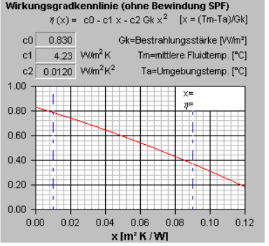
The trend of the curve can be described by means of a polynomial of the second order, clearly determined by means of three parameters, c0, c1 and c2 (or by means of η0, a1, a2; values measured at a wind velocity of 2-4 m/s):
\(\eta(x) = \ c_{0} – \left( c_{1} \cdot x \right) – (c_{2} \cdot G_{k} \cdot x^{2})\)
c0 is the efficiency rate achieved when the average temperature of the collector and the outdoor temperature are equal. This value should be as high as possible. c1 and c2 are a combination of different loss factors. In a well insulated collector, these values should be as low as possible.
The operation of a solar energy system requires a certain compromise. On one hand you need a collector to work at the highest efficiency level, on the other the generated hot water should have a temperature of 50°-60°C. This means inevitably having the collector operate at these temperatures.
This explains why solar energy is often used for the pre-heating of water in large buildings. When cold water is heated from 10°C to 30°C, the collector works at a high level of efficiency. In terms of energy demand, it is of little importance that the water is heated from 10 to 30°C or from 30 to 50°C. Therefore the efficiency rate of collectors is quite high in pre-heating. These kinds of systems can be profitable already after a few years.
As briefly outlined, there are three main collector categories. They are distinguished among other specifications by their efficiency rate curves.
- Glass-covered flat-plate collectors: c0 = 0.75-0.85, c1 = 3-6 W/m2/K
- Tube collectors: c0 = 0.65-0.80, c1 = 1-2 W/m2/K
- Unglazed (uncovered) collectors: c0 = 0.90-0.95, c1 = 10 W/m2/K
The illustration shows the most efficient models of these three types of collectors:
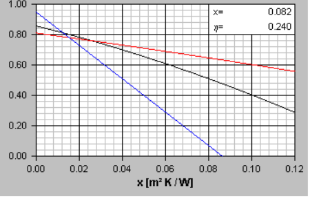
A value of x = 0.10 m2 K/W corresponds at an irradiance of 800 W/m2 to a temperature difference of \(T_{m} – T_{a} = 80\ {^\circ}C\). At these operating conditions, the indicated tube collector still has an efficiency rate of 60%, the covered collector 40%, while the unglazed collector is no longer able to produce energy at these temperatures.
Numeric Model for Non-Covered Collectors
In accordance with the standards for measurement (EN 12975) non-covered collectors are given an additional parameter. The efficiency function curve has the following form:
\(\eta = \eta_{0}*\left( 1 – b_{u}*u \right) – \frac{\left( b_{1} + b_{2}*u)*(t_{m} – t_{a} \right)}{G”}\)
The coefficients η0, bu, b1 and b2 are calculated by means of the adaption of the curve. G” is the total irradiance which is determined on the basis of the following equation:
\(G^{”} = G_{k} + (\frac{\varepsilon}{\alpha})(E_{L} – \ {\sigma T}_{a}^{4})\)
EL is the measurement of the intensity of long–wave irradiance onto the collector area and Ta is the outdoor temperature. For ε/α the value is fixed at 0.85, if the supplier has not given other indications.
Input Parameters
The decisive parameters that describe the efficiency of a collector, include in addition to the absorber area A, efficiency rate parameters c0, c1 and c2 and the IAM values KCH1 and KCH2, the specific heat capacity of the collector. The latter measures the “thermal inertia” of the collector: if a collector has great heat capacity it lasts longer, up until a certain quantity of solar irradiation has heated up the collector. On the other hand the collector still passes heat to the fluid when the sun is covered by a cloud. A collector with little heat capacity reacts more quickly to the variations of irradiation intensity.
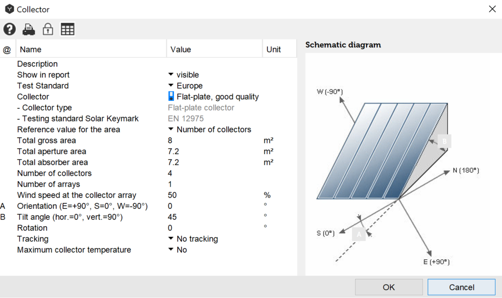
In many cases the orientation of the collector is established on the basis of the pitch and the orientation of the roof. Here one can ask if the collector should be oriented east or west (if south is not possible) or if it should be integrated into the facade. With flat roofs, orientation and tilt angle can be chosen freely. The question to ask in these cases is ‘With which angle is it possible to obtain the maximum annual efficiency?’ There is no single answer. The optimum orientation and tilt angle could be different according to water consumption, the size of the tank, the climate and many other conditions.
For the choice of orientation, Polysun makes available the following dialogue window:
Collector Data Entry in Polysun according to European Standards
Table: Collector data entry in Polysun in accordance with European standards
| Collector type: | Chapter 4.1 describes two different models to calculate the efficiency value of the collector. For the input “flat-plate or tube collector” the standard model will apply whilst for unglazed collectors the “uncovered collector” model will apply. |
| Eta0 laminar (1); bu: | “Eta0 laminar” is the efficiency value of a collector operating at outdoor temperature and in laminar flow conditions. Values of Eta0 laminar up to and of a2 refer to the aperture area of the collector and are determined at a radiation intensity of 800W/m2. “bu” is the wind reduction coefficient for uncovered collectors. |
| Eta0 turbulent: | The efficiency value of a collector operating at outdoor temperature and in turbulent flow conditions. |
| A1 (without wind) (2); b1: | A1 coefficient for flat-plate and tube collectors measured with no wind or b1 in uncovered collector models. |
| A1 (with wind) ; b2: | A1 coefficient for flat-plate and tube collectors measured in normal ventilation conditions or b2 for uncovered collector models. |
| A2 ; epsilon/alpha (3): | A2 coefficient for flat-plate and tube collectors or epsilon/alpha or uncovered collector models. |
| Dynamic heating capacity (4): | Value computed pursuant to EN 12975-2, section 6.1.6.2 |
| Nsis-Axis: | The orientation (tubes at a 90° horizontal or vertical elevation) for tube collectors. Mostly irrelevant in case of flat-plate collectors. |
| IAM model: | The “Ambrosetti Model” (described in chapter 1.3) is used to interpolate different flat-plate collectors. Tube collectors are interpolated by means of a cubic spline. |
| Angle factors (5): | IAM data are read over a table. Azimuth φ and elevation θ are described in chapter 1.3. |
| Volume: | Measured value of fluid volume in the collector including the manifold tubes. |
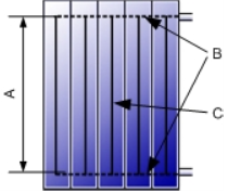
| Internal diameter: | Internal diameter of heat transfer pipes in the collector. C in figure n. 17. |
| Single pipe length (6): | The length of a single heat transfer pipe in the collector. A in figure n. 17. |
| Parallel piping: | Number of parallel pipings in the collector. 5 in figure n. 17. |
| Pipe roughness: | Roughness factor relating to the inner side. |
| Linear form factor: | The form factor of a pipe ranges based on bend radius between 1-1.5. The factor for rectilinear pipes is 1. |
| Friction factor: | The friction factor refers to pressure drops in branchings, valves, etc. If not measured it will be set on zero. |
| Test flow rate (7): | Fluid flow rate during a test. In l/h and collector. |
(1): In the event that no indications are available about Eta0 laminar ,Eta0 turbulent = Eta0 laminar will apply.
(2): Pursuant to new provisions the a 1 with wind coefficient is detected at a wind speed of 3 m/s. The efficiency parameter c1 may be worked out as follows:
\(c_{1} = a_{1\ without\ wind} + \frac{\left( a_{1\ with\ wind} – \ a_{1\ without\ wind} \right)}{(3\ m/s)} \cdot \ v_{wind} \cdot \ windportion\)
If a 1 without wind is not expressly indicated, select a 1 without wind 10% lower than a 1 with wind for flat-plate collectors and 5% lower for tube collectors.
(3): Fix epsilon/alpha = 0.85 in case this was not otherwise pre-set by the manufacturer.
(4): Directive EN 12975-2 establishes two different procedures for the calculation of dynamic heat capacity; in appendix J3 a measured value and in section 6.1.2.1 a calculated value. The calculated value is typically much lower than the measured value. Collector geometry is not taken into consideration. Notwithstanding the high reliability of the measured value the calculated value is actually used in Polysun.
(5): Angle factor tables may not yet be entered directly by the user. In the creation of a given collector a collector with similar IAM values should be copied.
(6): In case no measurable or obvious indication is given enter the width or length of the absorber.
(7): Test flow rate, maximum flow rate, maximum pressure and maximum temperature do not currently affect the calculation.